library(pacman)
p_load(
  janeaustenr,    # Contains the complete text of Jane Austen's novels
  tidyverse,
  tidytext,
  textdata,       # Contains sentiment lexicons (dictionaries)
  syuzhet         # For downloading the NRC lexicon
)

# Get the sentiment lexicons first
afinn_lex <- get_sentiments("afinn")
bing_lex <- get_sentiments("bing")

# Get NRC lexicon from syuzhet
nrc_lex <- get_sentiment_dictionary(dictionary = "nrc") %>%
           filter(!sentiment %in% c("positive","negative")) %>%
           select(-value,-lang)

# Prepare Austen's novels for analysis
austen_books <- austen_books() %>%      # Get all of Austen's novels
  group_by(book) %>%                    # Group the text by book title
  mutate(
    # Add line numbers (row_number() counts rows from 1 to n)
    linenumber = row_number(),
    chapter = cumsum(str_detect(text, regex("^chapter [\\divxlc]", ignore_case = TRUE))) # Add chapter number
  ) %>%
  ungroup() # Remove the grouping (so future operations aren't grouped by book)

austen_words <- austen_books %>%
unnest_tokens(word, text) §7 Sentiment Analysis 😊😐😢
- 📊 Understand the concept of sentiment analysis and its applications in Digital Humanities
- 🧮 Learn about different approaches to sentiment analysis
- Implement basic sentiment analysis using R
- 📈 Visualize sentiment patterns in literary texts
1 What is Sentiment Analysis? 🤔
Sentiment analysis, also known as opinion mining, is a technique used to determine the emotional tone behind a body of text. It’s a powerful tool in Digital Humanities for understanding the emotional content of literary works, historical documents, social media posts, and more.
1.1 Sentiment Analysis in Digital Humanities
In Digital Humanities, sentiment analysis offers several benefits:
- Scale: Analyze emotional patterns across large corpora of texts.
- Objectivity: Provide a systematic approach to studying emotions in text.
- Comparative Analysis: Compare emotional tones across different authors, time periods, or genres.
- Emotional Arc Analysis: Study how emotions change throughout a narrative.
- Cultural Insights: Explore emotional expressions in different cultural contexts.
1.2 Approaches to Sentiment Analysis
There are several approaches to sentiment analysis:
- Lexicon-based: Uses pre-defined dictionaries of words associated with positive or negative sentiments.
- Machine Learning: Trains models on labeled data to predict sentiment.
- Rule-based: Uses a set of manually crafted rules to determine sentiment.
- Hybrid: Combines multiple approaches for more accurate results.
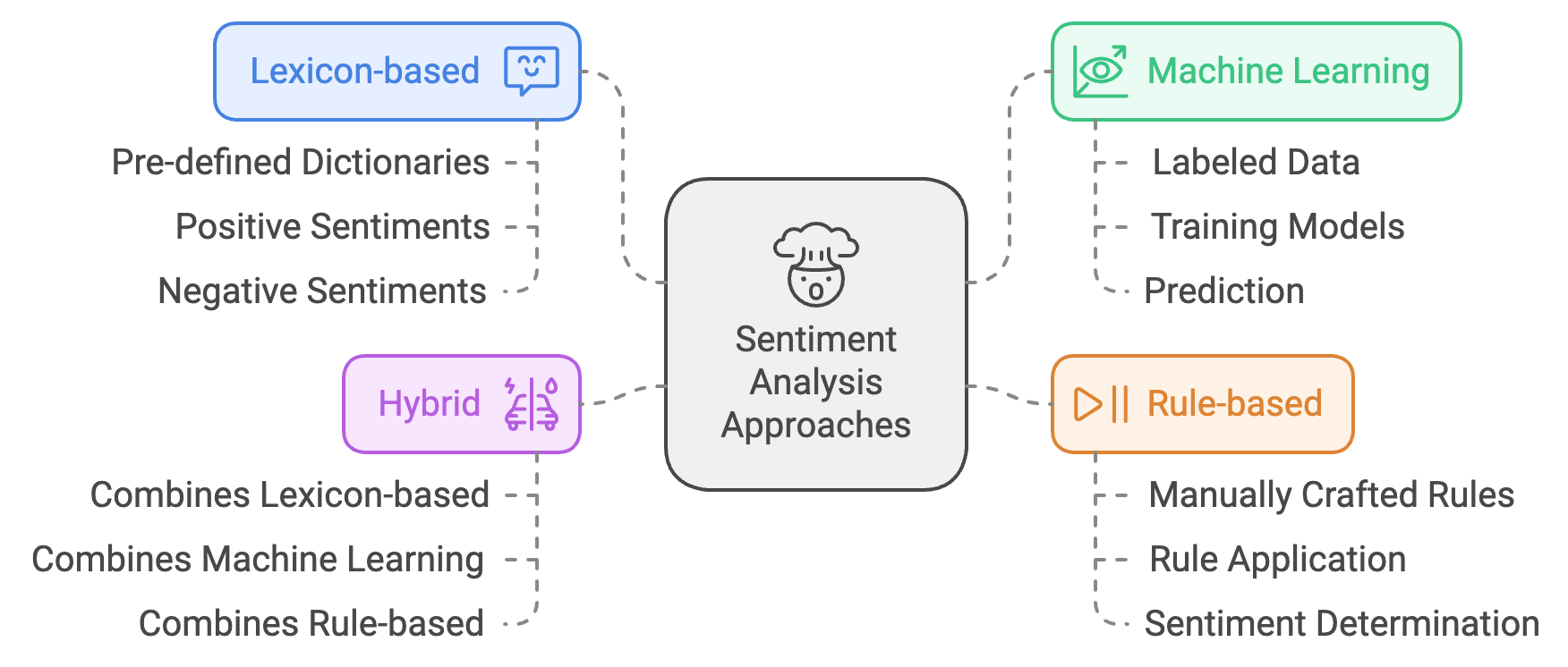
In this chapter, we’ll focus on the lexicon-based approach using the tidytext package in R.
2 Understanding Lexicon-Based Sentiment Analysis 📚
Lexicon-based sentiment analysis is like having an emotional dictionary that helps us understand the feelings expressed in a text. Let’s explore this concept through hands-on examples!
2.1 Try It Yourself: Basic Sentiment Tagging 🏷️
Before computers can analyze sentiment, they need a dictionary that tells them which words express positive or negative emotions. But creating such a dictionary isn’t straightforward! Even humans often disagree about whether a word is positive, negative, or neutral.
- Sentiment Dictionary (or Lexicon): A pre-defined list of words with their associated emotional values
- Tagging: The process of labeling words with their emotional values (positive, negative, or neutral)
- Sentiment Value: The emotional weight assigned to a word (e.g., “happy” = positive, “sad” = negative)
Let’s experience this challenge firsthand. In the exercise below, you’ll act as a “human lexicon creator 🕵️” tagging words just like we do when building sentiment dictionaries. Work with a partner to discover why this fundamental step of sentiment analysis is more complex than it might seem.
Comparing Sentiment Judgments 👥
Part 1: Individual Tagging
- Each student: Tag the following words as positive (😊), neutral (😐), or negative (😢)
- Write down your choices on paper or in a document
- Don't show your partner until you're both done!
Part 2: Compare & Discuss
- Find a partner and compare your choices
- Discuss words where you disagreed
- Consider: Why might you have tagged them differently?
Word 1 of 8
"dark"
How would you classify this word's sentiment?
Your Sentiment Dictionary:
If humans disagree on word sentiment, imagine how challenging it is for computers! Let’s look at some examples:
-
Multiple Meanings & Context
- “dark”: Could be negative (mood) or neutral (description)
- “cold”: Could be negative (feeling) or neutral (temperature)
- “bright”: Could be positive (mood) or neutral (light level)
-
Slang & Modern Usage
- “killing”: Could be negative (harm) or positive slang (“killing it” = doing well)
- “wild”: Could be positive (exciting) or negative (dangerous)
-
Subjective Interpretation
- “simple”: Could be positive (clear, elegant) or negative (unsophisticated)
- “quiet”: Could be positive (peaceful) or negative (lonely)
- “deep”: Could be neutral (measurement) or positive (profound)
These ambiguities demonstrate why:
- Context is crucial for understanding meaning
- Cultural and temporal differences affect interpretation
- Even “simple” words can have complex meanings
- Automated sentiment analysis needs sophisticated approaches to handle these nuances
2.2 Common Sentiment Lexicons 📖
After seeing how challenging it is to create sentiment dictionaries, let’s look at some widely-used lexicons in Digital Humanities research:
-
AFINN: A simple lexicon that rates words from -5 (very negative) to +5 (very positive)
- Example: “superb” = +5, “catastrophic” = -4
- Good for: Quick analysis, clear numerical scores
- Limitation: Misses nuanced emotions
-
Bing: Categorizes words as either positive or negative
- Example: “good” = positive, “bad” = negative
- Good for: Binary sentiment analysis
- Limitation: No neutral category or intensity levels
-
NRC: Classifies words into eight basic emotions plus positive/negative
- Emotions: anger, fear, anticipation, trust, surprise, sadness, joy, disgust
- Example: “birthday” → joy, anticipation, positive
- Good for: Detailed emotional analysis
- Limitation: More complex to interpret
2.2.1 Try It Yourself: Comparing Lexicons 🔍
Let’s explore how each lexicon works through a collaborative exercise:
-
Individual Tagging
- Work independently to tag the words below using each lexicon
- Keep your answers private until everyone is done
- Try to justify your choices as you go
-
Group Discussion
- Form groups of 2-3 students
- Compare your tags with your groupmates
- Discuss where and why your tags differed
- What factors influenced your decisions?
Let’s begin with the interactive tagging exercise below:
Your AFINN Tags:
- Compare how the same word might be tagged differently in each lexicon
- Notice how AFINN’s numerical scale captures intensity
- See how Bing’s simplicity makes quick classification easier
- Explore how NRC reveals emotional complexity
-
Which lexicon would you choose for analyzing:
- Movie reviews?
- Historical documents?
- Social media posts?
What are the trade-offs between simplicity and detail?
How might cultural or temporal differences affect these lexicons?
-
Choosing Lexicons for Different Contexts:
-
Movie Reviews: AFINN might be most suitable because:
- Its -5 to +5 scale captures intensity of opinions
- Reviews often use strong emotional language
- Numerical scores align well with star ratings
-
Historical Documents: Bing might work better because:
- Binary classification is less likely to misinterpret archaic language
- Simpler positive/negative distinction suits formal writing
- Less affected by changes in emotional intensity over time
-
Social Media Posts: NRC would be ideal because:
- Captures nuanced emotions like joy, anger, surprise
- Suits informal, emotionally expressive language
- Better at handling modern slang and emoji contexts
-
-
Trade-offs Between Simplicity and Detail:
-
Simple Lexicons (e.g., Bing)
- ✅ Easier to implement and interpret
- ✅ More robust across different contexts
- ❌ Miss nuanced emotional expressions
- ❌ Can’t capture intensity of sentiment
-
Complex Lexicons (e.g., NRC)
- ✅ Richer emotional analysis
- ✅ Better for nuanced interpretation
- ❌ More computationally intensive
- ❌ Higher risk of misclassification
-
Simple Lexicons (e.g., Bing)
-
Cultural and Temporal Impacts:
-
Cultural Differences
- Words may have different emotional connotations across cultures
- Metaphors and idioms might not translate emotionally
- Cultural context affects interpretation of neutral vs. emotional language
-
Temporal Changes
- Word meanings and emotional associations evolve over time
- Modern lexicons might misinterpret historical usage
- Slang and informal language constantly create new emotional expressions
-
Cultural Differences
3 Implementing Sentiment Analysis in R 💻
Let’s start with a practical example using Jane Austen’s novels. Let’s first download all the necessary data for our analysis.
The line chapter = cumsum(str_detect(text, regex("^chapter [\\divxlc]", ignore_case = TRUE))) breaks down into several parts:
-
Finding Chapter Headers:
regex("^chapter [\\divxlc]")-
^means “start of line” (NOT negation here!) -
chapterlooks for the word “chapter” -
[\\divxlc]looks for Roman numerals (I, V, X, etc.)
-
-
Different Uses of
^:- At start of pattern (
^chapter): means “starts with chapter” - Inside brackets (
[^abc]): means “NOT these letters”
Examples:
^chapter matches: [^chapter] matches: "Chapter 1" ✓ "dog" ✓ (d is not in 'chapter') "The Chapter" ✗ "cat" ✗ (c is in 'chapter') - At start of pattern (
-
Counting Chapters:
-
str_detect()returns TRUE/FALSE for each line -
cumsum()adds up these TRUEs (1) and FALSEs (0)
Example:
Text: str_detect(): cumsum(): "Chapter I" TRUE 1 "Some text..." FALSE 1 "Chapter II" TRUE 2 "More text..." FALSE 2 -
This creates a column that shows which chapter each line belongs to.
3.1 AFINN Analysis
# Summative Analysis for AFINN
afinn_summary <- austen_words %>%
  inner_join(afinn_lex, by = "word", relationship = "many-to-many") %>%  # Match words with their sentiment scores
  group_by(book) %>%                                                     # Group all words by book
  summarise(
    mean_sentiment = mean(value),                                        # Average sentiment per book
    total_words = n(),                                                   # Count of sentiment-scored words
    most_negative = min(value),                                          # Most negative score
    most_positive = max(value)                                           # Most positive score
  )

afinn_summary
# A tibble: 6 × 5
book mean_sentiment total_words most_negative most_positive
<fct> <dbl> <int> <dbl> <dbl>
1 Sense & Sensibility 0.426 7762 -5 4
2 Pride & Prejudice 0.508 7783 -4 4
3 Mansfield Park 0.521 10645 -4 4
4 Emma 0.535 10901 -4 4
5 Northanger Abbey 0.432 5066 -4 4
6 Persuasion 0.550 5130 -4 4# Emotional Arc for AFINN
afinn_arc <- austen_words %>%
inner_join(afinn_lex, by = "word") %>%
group_by(book, index = linenumber %/% 100) %>% # Group into chunks of 100 lines
summarise(sentiment = mean(value), .groups = "drop") # Average sentiment per chunk
afinn_arc# A tibble: 738 × 3
book index sentiment
<fct> <dbl> <dbl>
1 Sense & Sensibility 0 0.612
2 Sense & Sensibility 1 0.727
3 Sense & Sensibility 2 0.593
4 Sense & Sensibility 3 0.705
5 Sense & Sensibility 4 1.29
6 Sense & Sensibility 5 1.25
7 Sense & Sensibility 6 0.534
8 Sense & Sensibility 7 0.509
9 Sense & Sensibility 8 0.818
10 Sense & Sensibility 9 1.5
# ℹ 728 more rows# Plot AFINN results
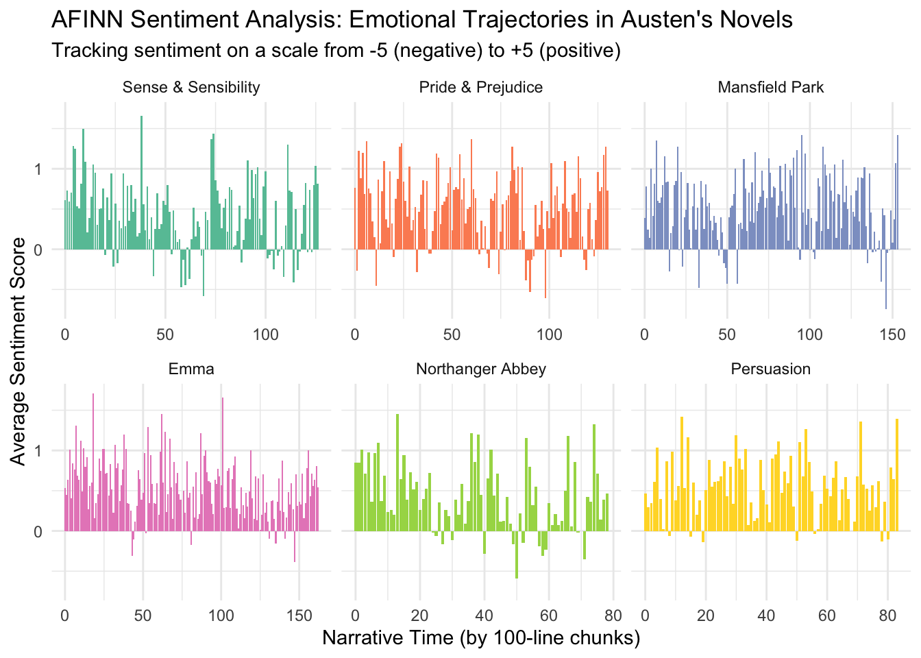
ggplot(afinn_arc, aes(x = index, y = sentiment, fill = book)) +
geom_col() +
facet_wrap(~book, scales = "free_x") +
theme_minimal() +
scale_fill_brewer(palette = "Set2") +
theme(legend.position = "none") +
labs(
title = "AFINN Sentiment Analysis: Emotional Trajectories in Austen's Novels",
subtitle = "Tracking sentiment on a scale from -5 (negative) to +5 (positive)",
x = "Narrative Time (by 100-line chunks)",
y = "Average Sentiment Score"
) 
%/%)
-
What is
%/%?- It’s integer division that always rounds down (floor division)
- Different from regular division (
/) which gives decimals - Different from ceiling (rounding up) or rounding to nearest integer
-
Examples:
# Regular division (/)     Floor division (%/%)
5 / 2  = 2.5             5 %/% 2 = 2
7 / 3  = 2.333...        7 %/% 3 = 2
-5 / 2 = -2.5           -5 %/% 2 = -3  (rounds down!)

# In our text analysis:
linenumber %/% 100 creates chunks:
1-99     %/% 100 = 0  (first chunk)
100-199  %/% 100 = 1  (second chunk)
200-299  %/% 100 = 2  (third chunk)
This helps us group lines of text into equal-sized chunks for analysis.
3.2 Bing Analysis
# Summative Analysis for Bing
bing_summary <- austen_words %>%
  inner_join(bing_lex, by = "word", relationship = "many-to-many") %>%  # Note: Discuss why we need to add "many-to-many" relationships
  count(book, sentiment) %>%  # Count positive and negative words
  pivot_wider(names_from = sentiment, # Reshape to have positive/negative columns
              values_from = n,
              values_fill = 0) %>%
  mutate(
    total_words = positive + negative,  # Total words with sentiment
    sentiment_ratio = positive / negative,  # Ratio of positive to negative
    net_sentiment = positive - negative  # Net sentiment (positive minus negative)
  )

bing_summary
# A tibble: 6 × 6
book negative positive total_words sentiment_ratio net_sentiment
<fct> <int> <int> <int> <dbl> <int>
1 Sense & Sensibili… 3671 4933 8604 1.34 1262
2 Pride & Prejudice 3652 5052 8704 1.38 1400
3 Mansfield Park 4828 6749 11577 1.40 1921
4 Emma 4809 7157 11966 1.49 2348
5 Northanger Abbey 2518 3244 5762 1.29 726
6 Persuasion 2201 3473 5674 1.58 1272# Emotional Arc for Bing
bing_arc <- austen_words %>%
inner_join(bing_lex, by = "word") %>%
count(book, index = linenumber %/% 100, sentiment) %>%
pivot_wider(names_from = sentiment,
values_from = n,
values_fill = 0) %>%
mutate(net_sentiment = positive - negative) Warning in inner_join(., bing_lex, by = "word"): Detected an unexpected many-to-many relationship between `x` and `y`.
ℹ Row 435434 of `x` matches multiple rows in `y`.
ℹ Row 5051 of `y` matches multiple rows in `x`.
ℹ If a many-to-many relationship is expected, set `relationship =
"many-to-many"` to silence this warning.bing_arc# A tibble: 738 × 5
book index negative positive net_sentiment
<fct> <dbl> <int> <int> <int>
1 Sense & Sensibility 0 20 47 27
2 Sense & Sensibility 1 22 54 32
3 Sense & Sensibility 2 16 35 19
4 Sense & Sensibility 3 20 45 25
5 Sense & Sensibility 4 21 63 42
6 Sense & Sensibility 5 25 63 38
7 Sense & Sensibility 6 39 44 5
8 Sense & Sensibility 7 23 31 8
9 Sense & Sensibility 8 15 39 24
10 Sense & Sensibility 9 22 63 41
# ℹ 728 more rows# Plot Bing results
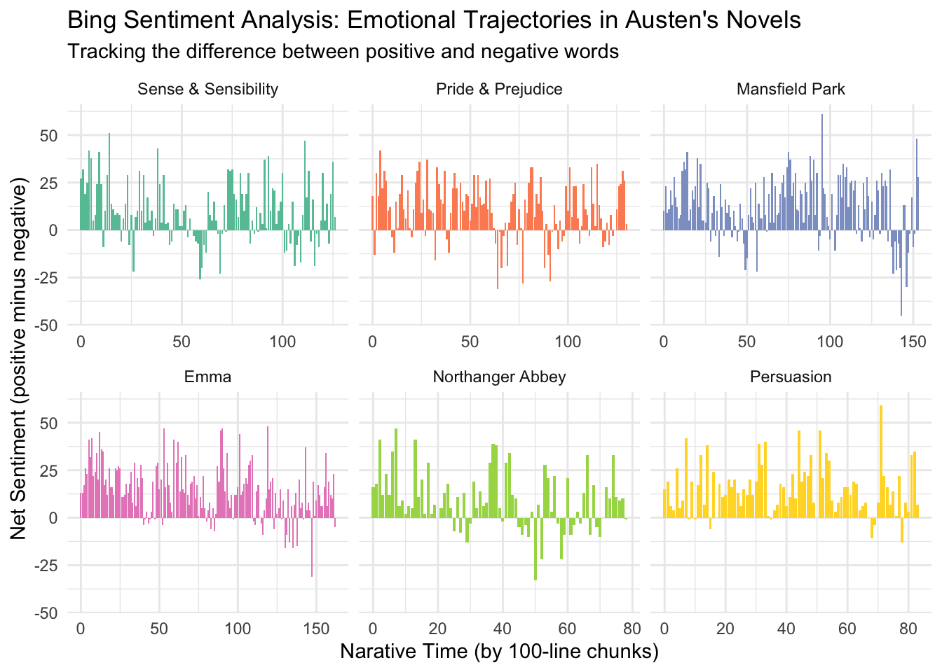
ggplot(bing_arc, aes(x = index, y = net_sentiment, fill = book)) +
geom_col() +
facet_wrap(~book, scales = "free_x") +
theme_minimal() +
scale_fill_brewer(palette = "Set2") +
theme(legend.position = "none") +
labs(
title = "Bing Sentiment Analysis: Emotional Trajectories in Austen's Novels",
subtitle = "Tracking the difference between positive and negative words",
x = "Narative Time (by 100-line chunks)",
y = "Net Sentiment (positive minus negative)"
) 
3.3 NRC Analysis
# Summative Analysis for NRC
nrc_summary <- austen_words %>%
  inner_join(nrc_lex, by = "word", relationship = "many-to-many") %>%
  count(book, sentiment) %>%                                           # Count words in each emotion category
  group_by(book) %>%
  mutate(proportion = n / sum(n)) %>%                                 # Calculate proportion of each emotion
  ungroup()

nrc_summary
# A tibble: 48 × 4
book sentiment n proportion
<fct> <chr> <int> <dbl>
1 Sense & Sensibility anger 1343 0.0697
2 Sense & Sensibility anticipation 3698 0.192
3 Sense & Sensibility disgust 1172 0.0608
4 Sense & Sensibility fear 1861 0.0966
5 Sense & Sensibility joy 3341 0.173
6 Sense & Sensibility sadness 2064 0.107
7 Sense & Sensibility surprise 1589 0.0825
8 Sense & Sensibility trust 4199 0.218
9 Pride & Prejudice anger 1295 0.0699
10 Pride & Prejudice anticipation 3596 0.194
# ℹ 38 more rows# Emotional Arc for NRC
nrc_arc <- austen_words %>%
inner_join(nrc_lex, by = "word", relationship = "many-to-many") %>%
count(book, index = linenumber %/% 100, sentiment) %>%
group_by(book, index) %>%
mutate(proportion = n / sum(n)) # Proportion of each emotion per chunk
nrc_arc# A tibble: 5,899 × 5
# Groups: book, index [738]
book index sentiment n proportion
<fct> <dbl> <chr> <int> <dbl>
1 Sense & Sensibility 0 anger 10 0.0498
2 Sense & Sensibility 0 anticipation 40 0.199
3 Sense & Sensibility 0 disgust 12 0.0597
4 Sense & Sensibility 0 fear 9 0.0448
5 Sense & Sensibility 0 joy 36 0.179
6 Sense & Sensibility 0 sadness 20 0.0995
7 Sense & Sensibility 0 surprise 24 0.119
8 Sense & Sensibility 0 trust 50 0.249
9 Sense & Sensibility 1 anger 14 0.0660
10 Sense & Sensibility 1 anticipation 42 0.198
# ℹ 5,889 more rows# Plot NRC results (focusing on two contrasting emotions for clarity)
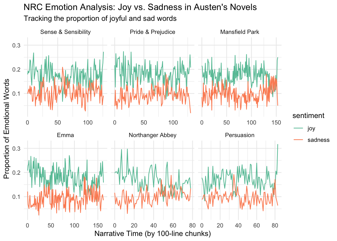
nrc_arc %>%
filter(sentiment %in% c("joy", "sadness")) %>% # Choose contrasting emotions
ggplot(aes(x = index, y = proportion, color = sentiment)) +
geom_line() +
theme_minimal() +
scale_color_brewer(palette = "Set2") +
facet_wrap(~book, scales = "free_x") +
labs(
title = "NRC Emotion Analysis: Joy vs. Sadness in Austen's Novels",
subtitle = "Tracking the proportion of joyful and sad words",
x = "Narrative Time (by 100-line chunks)",
y = "Proportion of Emotional Words"
) 
4 Character-Focused Analysis 🎭
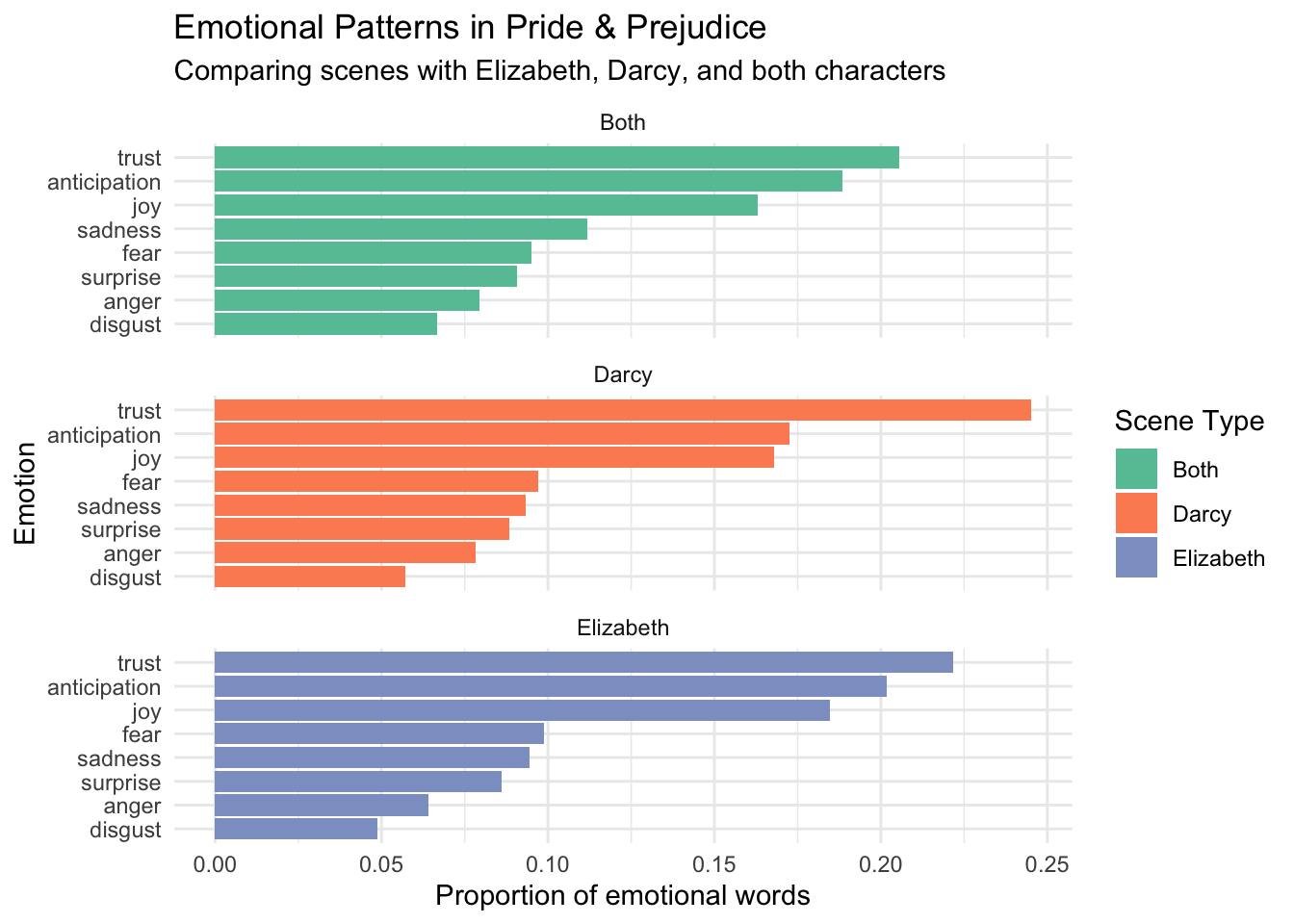
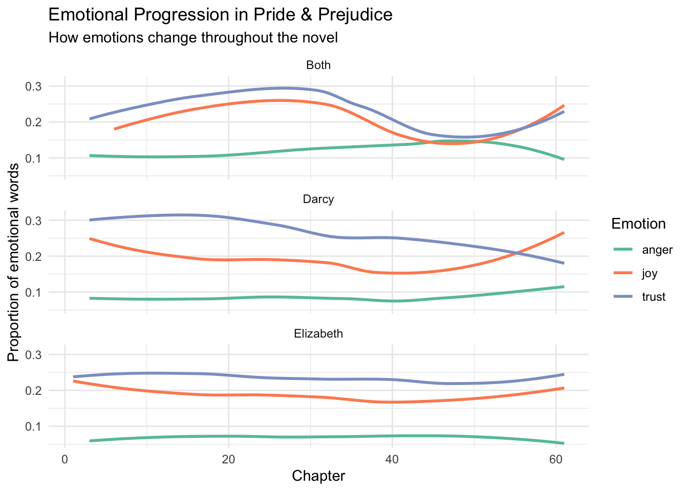
In addition to analyzing the sentiment in various novels, we can also conduct character-focused analysis. Let’s investigate some interesting questions about Jane Austen’s Pride and Prejudice using the methods we’ve learned.
4.1 Predict the Emotional Patterns 📊
Before we analyze the data, let’s make some predictions! Which emotions do you think dominate in different types of scenes?
While waiting for all votes to come in:
- Why did you choose these particular emotions for each scene type?
- Can you think of specific moments in the novel that support your predictions?
- How might the emotional patterns reflect the character development?
- Do you expect the emotional patterns to change over the course of the novel?
- Start Small: Begin with one book or character before comparing multiple ones
-
Visualize: Use
ggplotto see patterns - try both line plots and bar charts - Context Matters: Look at the actual text passages to verify your findings
- Compare Methods: Try the same analysis with different lexicons (AFINN, Bing, NRC)
Share your findings with classmates - different perspectives might reveal interesting patterns you hadn’t noticed!
5 Learning Check 🏁
1. What is the main purpose of sentiment analysis in Digital Humanities?
2. What is a key limitation of sentiment analysis in studying historical texts?
3. How does the AFINN lexicon differ from the Bing lexicon?
4. When we divide Austen's novels into 100-line chunks for analysis, what are we trying to understand?
5. What unique feature does the NRC lexicon offer compared to AFINN and Bing?
6 Conclusion
In this chapter, we’ve covered:
- Predicting and analyzing emotional patterns in Pride & Prejudice
- Using interactive polls to gather reader predictions about character emotions
- Comparing emotional patterns in scenes with Elizabeth, Darcy, and their interactions
- Visualizing how emotions change throughout the novel
- Understanding the limitations and possibilities of computational sentiment analysis
Our analysis of Pride & Prejudice demonstrates how computational methods can reveal emotional patterns in literary texts. Through both reader predictions and computational analysis, we’ve explored how emotions vary between characters and evolve throughout the narrative. The interactive polls allow us to compare human intuition with computational findings, highlighting both the strengths and limitations of sentiment analysis tools.
Remember that computational analysis is most powerful when combined with close reading and traditional literary analysis. The patterns we’ve discovered should spark questions and encourage deeper investigation of the text, rather than being treated as definitive conclusions.
Reader Predictions
Character Emotions
Emotional Arcs
Comparative Analysis
